Dynamic Compensation

Compensation techniques are used to improve system performance by shaping the dynamics. Among the most important methods are PD compensation, Lead compensation, PI compensation, and Lag compensation. Each method influences transient response, steady-state accuracy, and stability margins in different ways.

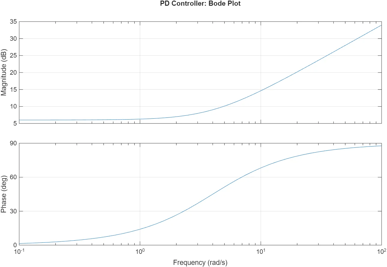
PD Compensation

The transfer function of a PD controller is:

D_c(s) = T_D s + 1

in frequency domain,

D_c(j\omega) = T_D j\omega + 1

where break frequency is:

\omega = \frac{1}{T_d}

Pros: It leads the phase, which means making the system respond faster.
Cons: Sensitive to high-frequency measurement noise.

Super wide

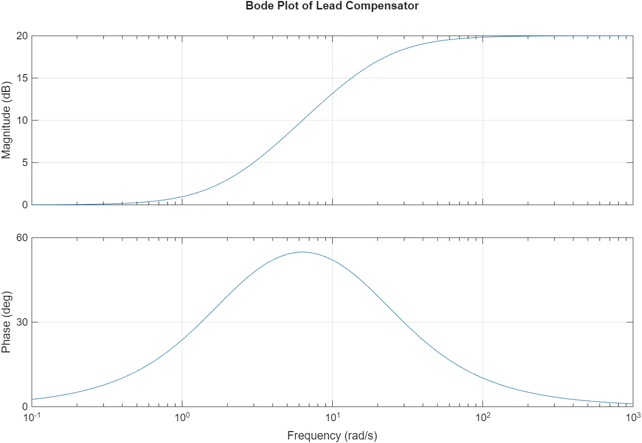
Lead Compensator

The transfer function of a lead compensator is:

D_c(s) = \frac{T_D s + 1}{\alpha T_D s + 1} \quad (\alpha < 1)

where break frequency is:

\omega = \frac{1}{T_D}, \qquad \omega = \frac{1}{\alpha T_D}

break frequency ‘αT_D’ is added.

Restrict high-frequency gain.
But also restrict ‘Phase Lead’ effect.

Super wide

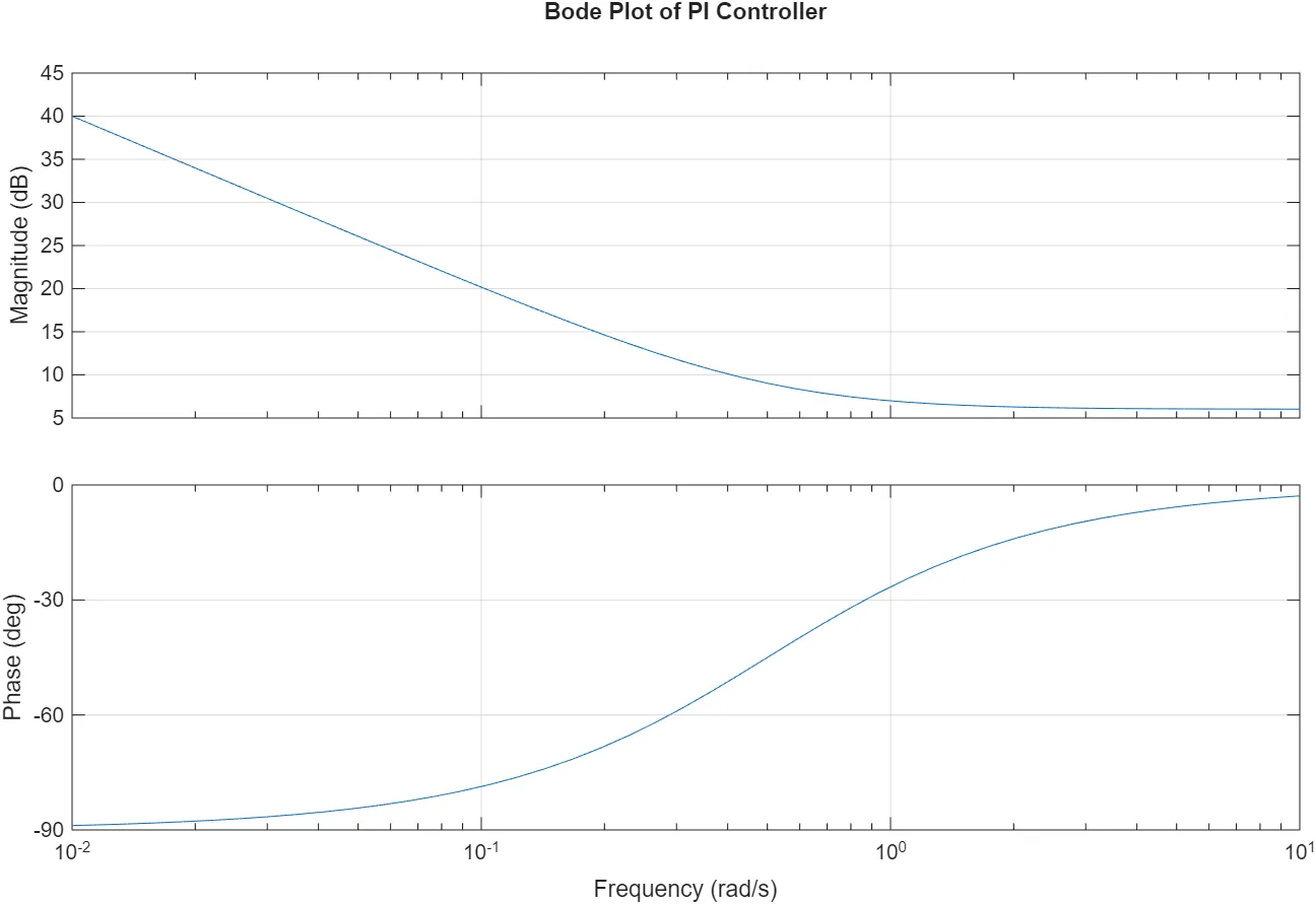
PI Compensation

The transfer function of a proportional–integral (PI) controller is:

D_c(s) = \frac{K}{s}(s + \frac{1}{T_I})

in frequency domain,

D_c(jw) = (\frac{k}{jw})(\frac{T_I jw+1}{T_I})

where break frequency is:

\omega = \frac{1}{T_I}

Pros: Infinite gain at the origin, which means eliminating steady-state error by increasing system order with adding pure integrator
Cons: May slow response on low-frequency area, especially at the origin

Super wide

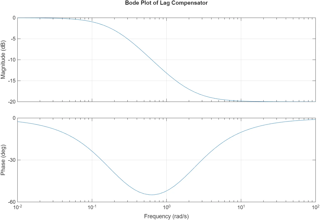
Lag Compensator

The transfer function of a lag compensator is:

D_c(s) = \alpha \frac{T_I s + 1}{\alpha T_I s + 1} \quad (\alpha > 1)

where break frequency is:

\omega = \frac{1}{\alpha T_I}, \qquad \omega = \frac{1}{T_I}

Unlike the PI controller, this one does not have a pole at the origin.

not likely PI controller, this does not have ‘s’ on 0.

It has a limited phase lag effect at low frequencies.
It also limits the amplification effect at low frequencies.
Depending on the design, phase lag can be applied only to specific frequency regions.
In frequency ranges where phase lag is not needed, other performance improvements are still possible.

Super wide

Summary

PD vs Lead: Both enhance transient performance.
- PD improves response speed but is noise-sensitive.
- Lead improves stability and robustness.
PI vs Lag: Both improve steady-state accuracy.
- PI completely eliminates steady-state error but may slow the system.
- Lag reduces steady-state error more gently while keeping transients intact.

Together, these compensation methods provide flexible tools for shaping system behavior in automatic control.

>> MATLAB Code