Low Pass Filter (LPF)

Introduction

This post introduces the Low Pass Filter (LPF) from a control systems perspective.

In electrical engineering, LPFs are commonly studied in signal processing or image processing courses.
They are typically used to attenuate high-frequency noise while preserving low-frequency components.

Rather than focusing on hardware implementations using R, L, and C components, this post explains LPF as a software-based recursive filter, building directly on moving average filters.

Review: Limitation of the Moving Average Filter

The moving average filter improves upon the simple average by considering only a recent window of data.

However, it has a critical limitation:

All samples within the window are treated equally.

Consider the sequence:

Assume a window size of $n=5$.

At time $k$, the window becomes:

The moving average assigns each value a weight of $1/5$.

But observe:

• 2 is 5 seconds old
• 3 is 4 seconds old
• 6 is the most recent measurement

Despite this, all samples contribute equally.

Motivation for Low Pass Filtering

In real systems, recent measurements are usually more informative than older ones.

A natural question arises:

What if we assign more weight to newer data?

For example, instead of computing

we could emphasize the most recent value:

This produces an estimate that reacts faster to changes while still suppressing noise.

Core Idea of the Low Pass Filter

A low pass filter can be interpreted as a weighted moving average, where newer samples receive higher importance.

In recursive form:

where:

• $\bar{x}_{k-1}$ is the previous filtered value
• $x_k$ is the current measurement
• $a$ is a weighting factor with $0 < a < 1$

The parameter $a$ controls how strongly the filter reacts to new data.

Comparison with Moving Average

• Moving Average
  Equal weights for all samples in the window

• Low Pass Filter
  Larger weight on recent samples
  Smaller weight on older information

This difference becomes increasingly important when:

• The signal changes rapidly
• The window size is large
• Tracking accuracy matters

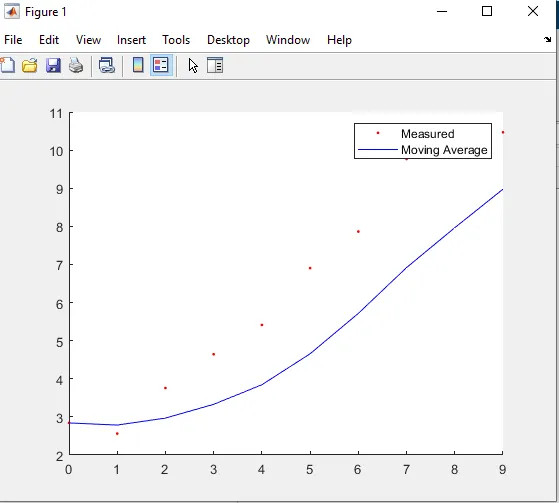
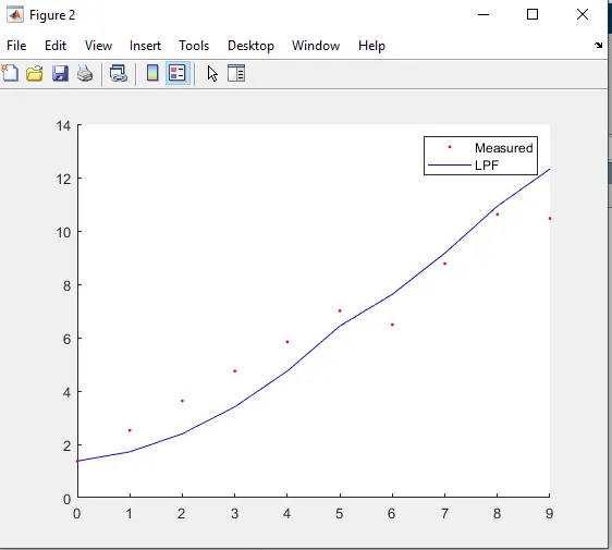
Visual Comparison Insight

When tracking a signal such as:

• Moving average exhibits noticeable lag
• Low pass filter follows the trend more closely

Even with a small number of samples, the improvement is visually apparent.

Practical Recursive Update

In implementation, LPF often appears as:

This form highlights that:

• The filter corrects the previous estimate
• The correction magnitude depends on $a$

This structure is fundamental in control and estimation theory.

Why This Matters

• LPF balances noise suppression and responsiveness
• It generalizes moving average filters
• It directly leads to Kalman filtering concepts

Choosing $a$ appropriately is critical:

• Small $a$ → smoother but slower response
• Large $a$ → faster response but more noise

Summary

• Moving average filters treat all samples equally
• Low pass filters emphasize recent measurements
• LPF reduces lag while maintaining noise suppression
• LPF forms the conceptual bridge to Kalman filters

Weighting recent information is the key to practical filtering.