· Hankyu Kim · Filter · 3 min read
Moving Average Filter
The moving average filter reduces noise while preserving the dynamic behavior of time-varying signals by averaging only a recent window of measurements.

Introduction
This post introduces the Moving Average Filter, an extension of the basic average filter designed to handle time-varying signals.
As shown in the previous post, taking an average is highly effective at removing noise.
However, when the underlying signal changes over time, a simple average filter becomes inadequate.
Limitation of the Average Filter
The standard average filter computes the mean of all past measurements.
This works well when the true value is constant, but fails when the signal evolves.
Consider a signal that increases linearly:
Applying a cumulative average produces:
Instead of following the signal, the filter outputs a smoothed but lagging estimate.
As the sequence grows longer, this accumulated lag becomes more severe.
Why Moving Average?
Most real-world signals are dynamic.
We want a filter that:
- Suppresses noise
- Responds to recent changes
- Does not accumulate long-term bias
This motivation leads to the Moving Average Filter.
Core Idea
Instead of averaging all past data, the moving average computes the mean over a fixed window of recent samples.
At time , only the most recent samples are used:
Old data is discarded, allowing the estimate to track changes in the signal.
Simple Example
Assume the input sequence:
Using a window size of :
Comparison:
| Measured | 1 | 2 | 3 | 4 | 5 |
|---|---|---|---|---|---|
| Average Filter | 1 | 1.5 | 2 | 2.5 | 3 |
| Moving Average | 1 | 1.5 | 2.5 | 3.5 | 4.5 |
Even in this simple case, the moving average tracks the signal far more accurately.
Dynamic Signal Example
Consider a signal defined as
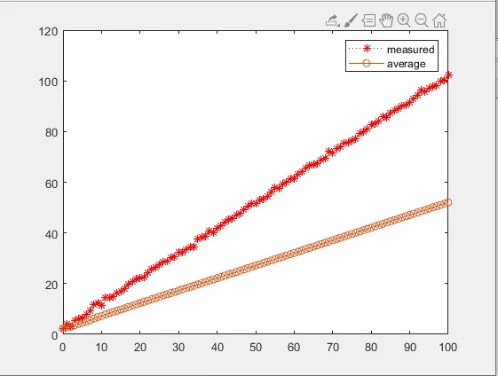
- The average filter increasingly lags behind the true signal
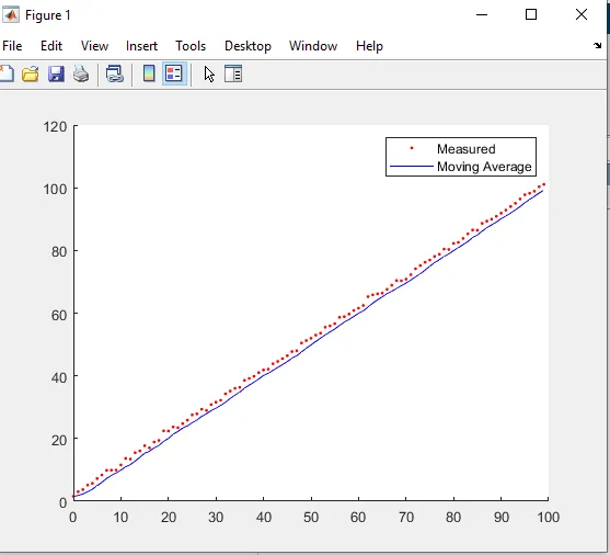
- The moving average filter continues to track the trend
Using a window of the most recent 5 samples, the moving average maintains stability while responding to changes.
The performance difference becomes more pronounced as:
- The signal duration increases
- The signal variation becomes larger
Efficient Recursive Update
The moving average can be updated efficiently without recomputing the full sum.
Let:
- be the previous moving average
- be the new sample
- be the oldest sample leaving the window
Then:
This update rule highlights the sliding window nature of the filter.
Key Insight
- Only the newest and oldest samples affect the update
- Middle samples remain unchanged
- The filter adapts quickly to signal changes
This structure provides a balance between noise reduction and responsiveness.
Why This Matters
- Average filters fail for time-varying signals
- Moving average filters preserve dynamics
- Window size controls the noise–responsiveness tradeoff
The moving average filter is a practical stepping stone toward more advanced adaptive filters.
Summary
- Moving average filters use a fixed window of recent data
- They remove noise without excessive lag
- They outperform cumulative averages on dynamic signals
- They are widely used in signal processing and control
Simple modification, significantly better behavior.


